Face Detection with Viola-Jones

Viola-Jones was introduced by Paul Viola and Michael Jones at ICCV (Viola & Jones, 2004) and CVPR (Viola & Jones, 2001) in 2001. You can find reviews and explanations everywhere. Still, I want to revisit it because it’s a great way for newer folks to see what computer vision was like two decades ago.

Viola-Jones face detection: How it works

Face detection, which is figuring out if there’s a face in an image, is different from face recognition, which is figuring out whose face it is. Think of face detection as a building block for more advanced face recognition systems. Instead of using one powerful classifier, Viola-Jones cleverly uses a bunch of simple, “weak” classifiers. These weak classifiers are built by finding the best thresholds for those Haar-like features you’ll see below. The algorithm then ranks and organizes these classifiers into a cascade to make the process super efficient.

The Viola-Jones algorithm showcases several tricks up its sleeve. First, it uses Haar-like features for feature extraction, speeding things up with the integral image concept. Then, it uses AdaBoost to select the most useful features from the huge set it generates. Finally, the cascade classifier design lets it quickly discard areas of the image that definitely don’t contain faces, making the whole process much faster.

Feature extraction: Haar-like features

Input: A 24x24 image that’s been normalized (zero mean, unit variance).

Output: A long, skinny vector (162,336 elements!) containing the values of all the Haar-like features.

This algorithm is a cool example of mixing traditional CV techniques with ML. Notice that for feature extraction, it doesn’t use fancy CNNs. Instead, it uses the intuitive Haar-like features.

Figure 1: The five types of Haar-like features

Basically, these features compare the sum of pixel intensities in black regions to the sum in white regions. The Viola-Jones method uses two-rectangle, three-rectangle, and four-rectangle features. Think of the four-rectangle feature as a kind of diagonal line detector. They’re called “Haar-like” because they’re similar to the +1/-1 square functions you find in Haar wavelets.

These features are surprisingly good at face detection. Why? Because things like eye sockets and cheeks often have clear dark/light boundaries, and features like the nose and mouth can be thought of as lines with a certain width.

Figure 2: Haar-like features applied on human face

The algorithm applies these “masks” to sliding windows that are 24x24 pixels. The paper calls this window a detector, and 24x24 is the base resolution of the detector. We’ll talk about where the detectors come from later. The five masks, starting from small sizes like 2x1, 3x1, 1x2, 1x3, and 2x2, all the way up to the size of the full detector (24x24), slide across the window. For example, a 2x1 edge mask will move across each row, then expand to 4x1 and move again… until it’s 24x1. Then it starts over from 2x2 to 24x2, then 2x3 to 24x3, and so on until it reaches 24x24.

Now, why is the output vector 162,336 elements long? A 24x24 image has 43,200, 27,600, 43,200, 27,600 and 20,736 features of category (a), (b), (c), (d) and (e) respectively, resulting in 162,336 total features.

Here’s a quick MATLAB snippet to calculate the total number of features. Note that some sources may say the total is 180,625. That’s because they use two four-rectangle features instead of just one.

frameSize = 24;
features = 5;
% All five feature types:
feature = [[2,1]; [1,2]; [3,1]; [1,3]; [2,2]];
count = 0;
% Each feature:
for ii = 1:features
    sizeX = feature(ii,1);
    sizeY = feature(ii,2);
    % Each position:
    for x = 0:frameSize-sizeX
        for y = 0:frameSize-sizeY
            % Each size fitting within the frameSize:
            for width = sizeX:sizeX:frameSize-x
                for height = sizeY:sizeY:frameSize-y
                    count=count+1;
                end
            end
        end
    end
end
display(count)

So, now we know how to define and extract features. But a few important details are still missing, which can be confusing for beginners!

Nitty-gritty Ahead

Here I’ll elaborate on how they set up the sliding windows, how they get rid off blank areas, and some performance issues.

Get detectors (sliding windows)

So where do these 24x24 “detectors” actually come from? A helpful video shows this process clearly.

The size of a face can vary greatly between photos (the original images discussed in the paper are 384x288 pixels). You can select the size of your sliding window empirically (making sure it’s at least 24x24) and resize it to a 24x24 detector.

The paper also suggests a more standardized approach: Scan the image with a fixed-size 24x24 detector. Instead of making the detector bigger, you shrink the image by a factor of 1.25 and scan it again. This creates a pyramid of image scales (up to 11 in the paper), each 1.25 times smaller than the last.

The 24x24 detector moves one pixel each step, horizontally and vertically. In the downsampled images, the equivalent moving step is larger. Thus, by downsampling, the image pyramid adjusts both the equivalent detector size and the step size.

Normalization before convolution

Before applying the Haar-like features, each 24x24 detector is normalized. This involves adjusting the pixel values so the image has a mean of zero and a variance of one. If a detector’s variance is below a certain threshold, it’s considered too “plain” and not likely to contain a face, so it’s skipped to save processing time.

Performance

Interestingly, you can actually get better detection performance by only using the two-rectangle and three-rectangle features (types (b) and (c) in Figure 2. Given the computational efficiency at that time, the whole image could be processed at up to 15 frames per second. Of course, with modern computers, it’s fine to just use all five Haar-like features!

Fasten convolution process: integral image

Input: An N x M image I

Output: An N x M integral image II

Remember those +1/-1 rectangles in the Haar-like features? It would take a long time to directly multiply the feature masks with all the pixels. That’s where the integral image comes in! It’s a clever way to replace the convolution (mask multiplication) with just a few additions.

Figure 3: An integral image (center) from a 4x4 image

In an integral image, each pixel at location $(x,y)$ stores the sum of all pixels above and to the left of it in the original image:

$$II(x,y)=\sum _{i=1}^x\sum _{j=1}^{y}I(i,j)$$

This simplified representation speeds up feature extraction drastically. Now, calculating the convolution of the five masks on one position only requires $1+2+1+2+4=10$ operations!

Feature selection: AdaBoost

Input: The feature vector $x$ and label $y$ (face or not face) for each training image (around 5,000 faces and 5,000 non-faces).

Output: A “strong” classifier $h(x)$ made up of $T$ “weak” classifiers $h_t(x)$, chosen from $T$ features.

AdaBoost is an algorithm that turns weak classifiers into a strong one. In this step, you’re training a classification function that decides whether an image contains a face or not. You use the Haar-like features we extracted and a training dataset of positive (faces) and negative (non-faces) examples (at least 5,000 of each). The illustration below helps understand the process.

Figure 4: The AdaBoost algorithm

Each time around, a “weak classifier” is chosen. Samples that were misclassified by the previous classifier get more weight, so the next classifier focuses on getting those right. By combining these “weak” classifiers (which, in this case, are based on simple image boundaries), we create a much stronger, more accurate classifier.

AdaBoost is often described as a forest of stumps. This analogy really captures the idea. AdaBoost stands for Adaptive Boosting. There are lots of boosting algorithms. Remember the random forest binary classifier? Each tree is built with random samples and several features from the full dataset. Then, the new sample is fed into each decision tree, getting classified, and the labels are collected to count the final result.

During the training process, the order doesn’t matter at all, and all the trees are equal. In the forest of stumps, all the trees are 1-level, calling stumps (only root and 2 leaves in binary classification problems). Each stump is a weak classifier using only 1 feature from the extracted features. First, we find the best stump with the lowest error. It will suck. A weak classifier is only expected to function slightly better than randomly guessing. It may only classify the training data correctly 51% of the time. The next tree will then emphasize the misclassified samples and will be given a higher weight if the last tree doesn’t go well.

Figure 5: The training process of a weak classifier

The algorithm from the [viola2001rapid] can be summarized as above. It’s adequate for a basic implementation of the algorithm, like this project.

Nitty-gritty Ahead

Despite this, there are still some details that merit the discussion. This includes how a stump is found and how to select the best stump.

Find decision stump by exhaustive search

Input: The $f$-th feature of all $n$ samples, the weights of all samples

Output: A weak classifier $h_t(x)$

So, we know how to combine a bunch of weak classifiers to make a strong one. But how do we actually find the best “decision stump” in the first place (the best $h_j(x)$ in step 2 of the loop in the AdaBoost algorithm shown in Figure 4)? This part is often glossed over in many projects (like this one) and even in the paper itself.

Luckily, a clear explanation I found helped me a lot (Wang, 2014). The resources mentioned in this post are listed in the References.

A single decision stump is constructed with 4 parameters: threshold, toggle, error, and margin.

Parameter	Symbol	Definition
Threshold	$\tau$	The boundary of decision.
Toggle	$\mathrm{T}$	Decide if it means +1 (positive) or -1 (negative) when $>\tau$.
Error	$\mathrm{E}$	The classification error after threshold and toggle are set up.
Margin	$\mathrm{M}$	The largest margin among the ascending feature values.

The exhaustive search algorithm of decision stumps takes the $f$-th feature of all the $n$ training examples as input, and returns a decision stump’s 4-tuple $\left\{\tau ,\mathrm{T},\mathrm{E},\mathrm{M}\right\}$.

First, since we need to compute the margin $\mathrm{M}$, the gap between each pair of adjacent feature values, the $n$ examples are rearranged in ascending order of feature $f$. For the $f$-th feature, we have

$$x_{f_1}\le x_{f_2}\le x_{f_3}\le ...\le x_{f_n}$$

, while $x_{f_n}$ is the largest value among the $f$-th feature of all $n$ samples. It doesn’t mean the $n$-th sample since they are sorted.

In the initialization step, $\tau$ is set to be smaller than the smallest feature value $x_{f_1}$. Margin $\mathrm{M}$ is set to 0 and error $\mathrm{E}$ is set to an arbitrary number larger than the upper bound of the empirical loss.

Inside the $j$-th iteration, a new threshold $\tau$ is computed, which is the mean of the adjacent values:

$$\hat{\tau }=\frac{x_{f_j}+x_{f_{j+1}}}{2}$$

And the margin is computed as:

$$\hat{\mathrm{M}}=x_{f_{j+1}}-x_{f_j}$$

We compute the error $\hat{\mathrm{E}}$ by collecting the weight $w_{f_j}$ of the misclassified samples.

Since the toggle is not decided yet, we have to calculate $erro{r}_{+}$ and $erro{r}_{-}$ for both situations. If $erro{r}_{+}<erro{r}_{-}$, then we decide that toggle $\hat{\mathrm{T}}=+1$, otherwise $\hat{\mathrm{T}}=-1$.

Finally, the tuple of parameters with smallest error is kept as $\left\{\tau ,\mathrm{T},\mathrm{E},\mathrm{M}\right\}$.

Figure 6: Decision stump by exhaustive search

Choose the best stump

Input: $d$ stumps for $d$ given features

Output: the best decision stump

During each training round $t$ in AdaBoost, a weak classifier $h_t(x)$ is selected. For each feature, we utilize the method in Find decision stump by exhaustive search to decide on the best parameter set for the decision stump. $1\le t\le T$, $T$ is the total number of weak classifiers, usually we let $T$ be the full length of the feature vector.

The best stump among all the stumps should have the lowest error $\mathrm{E}$. We select the one with the largest margin $\mathrm{M}$ when the errors happen to be the same. It then becomes the $t$-th weak classifier.

The weights assigned to all $n$ samples will be adjusted, and thus, the exhaustive search should be carried out again using the updated weights. The idea behind this part is quite straightforward.

Figure 7: Finding the parameters of the best stump

Figure 8: AdaBoost algorithm with the optimal $h_t(x)$

Fasten classification: cascade classifier

Input: Samples and features.

Output: A cascade classifier, where each step contains several weak classifiers.

The whole point of this cascade is to make the detection process really fast when you feed it a new image (like the 384x288 example from the paper). Most of the sub-windows you’re checking for faces will not contain faces, so we want to quickly discard them.

Think of this as an attentional cascade. We want to pay close attention to the parts of the image that might have faces, and ignore the rest.

Our goals are:

1. Throw out non-faces as early as possible to reduce computation.
2. Focus on those “hard” examples (false positives) because the easy negative samples were already removed.

Figure 9: Cascading

The cascade is built from a series of “stages” or “layers,” each made up of a few weak classifiers. Remember the “strong” classifier we built with AdaBoost in Feature selection AdaBoost? That’s just the sum of weighted votes from all the weak classifiers. You may use that directly for face detection, and some projects do exactly that way. But, as we said earlier, we shouldn’t use all those weak classifiers on every single detector, which will be very slow.

At each stage, we only use a subset of the weak classifiers, as long as we can guarantee a certain false positive rate and detection rate. In the next stage, only the positive and false-positive samples (the “hard” samples) are used to train the classifier. All we have to do is set the maximum acceptable false-positive rate and the minimum acceptable detection rate per layer, as well as the overall target false positive rate.

Figure 10: Building a cascade detector

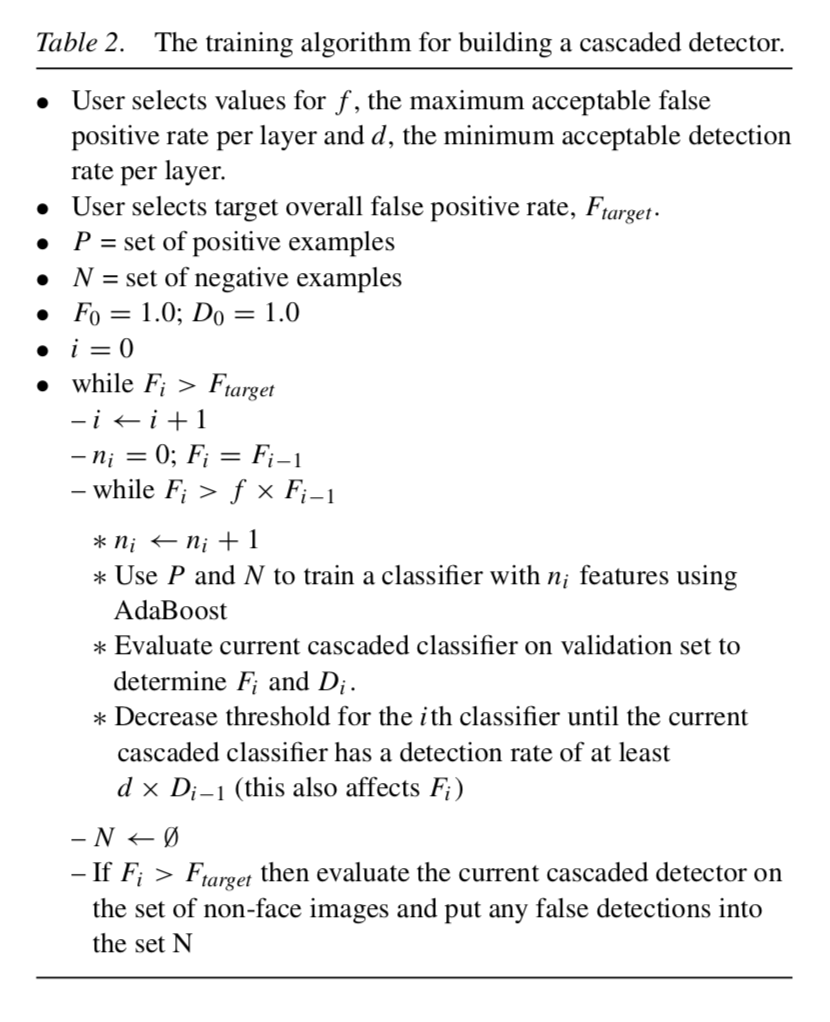
We iteratively add more features to each layer to achieve higher detection rates and lower false-positive rates until the requirements are met. Then we move on to the next layer. We create the final attentional cascade when the overall target false-positive rate is low enough.

Hope this explanation helps you better understand how the algorithm works!

Links

1. Rapid Object Detection using a Boosted Cascade of Simple Features
2. Haar-like feature - Wikipedia
3. Viola–Jones object detection framework - Wikipedia
4. Viola-Jones’ face detection claims 180k features - Stack Overflow
5. An Analysis of the Viola-Jones Face Detection Algorithm
6. AdaBoost, Clearly Explained - YouTube
7. GitHub - Simon-Hohberg/Viola-Jones: Python implementation of the face detection algorithm by Paul Viola and Michael J. Jones
8. Understanding and Implementing Viola-Jones (Part Two)

References

Viola, P., & Jones, M. (2001). Rapid object detection using a boosted cascade of simple features. Proceedings of the 2001 IEEE Computer Society Conference on Computer Vision and Pattern Recognition. CVPR 2001, 1, I–I.

Viola, P., & Jones, M. J. (2004). Robust real-time face detection. International Journal of Computer Vision, 57, 137–154.

Wang, Y.-Q. (2014). An analysis of the Viola-Jones face detection algorithm. Image Processing On Line, 4, 128–148.